Note

This page was generated from docs/notebooks/inversion/L_curve.ipynb.

L-curve criterion

By P.C. Hansen

Diffinition

Practically, in order to solve inversion problems \(Ax=b\) \((A\in\mathbb{R}^{m\times n}, x\in\mathbb{R}^n, b\in\mathbb{R}^m)\), we need to consider the similar form of least-squeares equations as follows:

\[\begin{split}\begin{align} x_\lambda &= \arg\min\{||Ax - b||_2^2 + \lambda\cdot||L(x - x_0)||_2^2\}\\ & = (A^\mathsf{T}A + \lambda L^\mathsf{T}L)^{-1} (A^\mathsf{T}b + \lambda L^\mathsf{T}x_0). \end{align}\end{split}\]

\(\lambda\in\mathbb{R}\) is a real regularization parameter that must be chosen by the user. The vector \(b\) is the given data and the vector \(x_0\in\mathbb{R}^n\) is a priori estimate of \(x\) which is set to zero when no a priori information is available. \(||Ax - b||_2\) is the residual term and \(||L(x - x_0)||_2\) is the regularization term, where \(L\in\mathbb{R}^{n \times n}\) is an operator matrix like a laplacian one. \(\lambda\) is the parameter which decides the contribution to these terms. And L-curve criterion is the method to balance between these contribution and optmize the inversion solution.

L-curve is precisely following points curve:

\[(||Ax - b||_2, ||L(x - x_0)||_2).\]

L-curve criterion is based on the fact that the optimal reguralization paramter is acheived when the L-curve point:

\[(\log||Ax_\lambda - b||_2,\; \log||L(x_\lambda - x_0)||_2)\]

lies on this corner.

In order to obtain the strict \(\lambda\) on the L-curve “corner” which is defined by the mathmatical method, we can calculate the L-curve carvature \(\kappa\) given by following equation:

\[\begin{split}\begin{align} \kappa &= \frac{f^{\prime\prime}(x)}{\left[1 + f^{\prime}(x)^2\right]^{3/2}}=-2 \eta\rho\frac{\lambda^2 \eta + \lambda \rho + \rho\eta/\eta^\prime}{(\lambda^2 \eta^2 + \rho^2)^{3/2}},\\ \rho &\equiv ||Ax_\lambda - b||_2^2,\\ \eta &\equiv ||L(x_\lambda - x_0)||_2^2,\\ \eta^\prime &\equiv \frac{d\eta}{d\lambda} \end{align}\end{split}\]

Using the singular value decomposion (SVD) fomula, \(x_\lambda\) is described as follows:

\[\begin{split}\begin{align*} x_\lambda &= (A^\mathsf{T}A + \lambda L^\mathsf{T}L)^{-1} A^\mathsf{T}b\\ &= L^{-1}((AL^{-1})^{\mathsf{T}}AL^{-1} + \lambda I_n)^{-1}(AL^{-1})^\mathsf{T}b\\ &= L^{-1}(V\Sigma^{\mathsf{T}} U^{\mathsf{T}}U\Sigma V^{\mathsf{T}} + \lambda I_n)^{-1} (U\Sigma V^{\mathsf{T}})^{\mathsf{T}}b \quad (\because AL^{-1} = U\Sigma V^{\mathsf{T}}: \text{using SVD})\\ &= L^{-1}V^{\mathsf{-T}}(\Sigma^{\mathsf{T}}\Sigma + \lambda I_r)^{-1}V^{\mathsf{-1}}V\Sigma^{\mathsf{T}}U^\mathsf{T}b\\ &= L^{-1}V(\Sigma^2 + \lambda I_r)^{-1}\Sigma U^\mathsf{T}b \quad (\because V^{-\mathsf{T}} = V, \Sigma = \Sigma^\mathsf{T} \in \mathbb{R}^{r\times r})\\ &= \tilde{V}(I_r + \lambda \Sigma^{-2})^{-1} \Sigma^{-1} U^\mathsf{T}b \quad (\because \tilde{V} \equiv L^{-1}V)\\ &= \tilde{V} W \Sigma^{-1} U^\mathsf{T} b\\ &= \tilde{V} \begin{pmatrix} w_1(\lambda)\frac{1}{\sigma_1} & & \\ & \ddots & \\ & & w_r(\lambda)\frac{1}{\sigma_r} \end{pmatrix} \begin{pmatrix} u_1^\mathsf{T}b \\ \vdots \\ u_r^\mathsf{T}b \end{pmatrix}\\ &= \begin{pmatrix} \tilde{v}_1 & \cdots & \tilde{v}_r \end{pmatrix} \begin{pmatrix} w_1(\lambda)\frac{u_1^{\mathsf{T}}b}{\sigma_1}\\ \vdots\\ w_r(\lambda)\frac{u_r^{\mathsf{T}}b}{\sigma_r} \end{pmatrix}\\ &= \sum_{i=1}^r w_i(\lambda) \frac{u_i^\mathsf{T}b}{\sigma_i}\tilde{v}_i, \end{align*}\end{split}\]

where,

\[\begin{split}\begin{align*} W &\equiv \text{diag}(w_1(\lambda),..., w_r(\lambda)),\\ w_i(\lambda) &\equiv \frac{1}{1 + \lambda/\sigma_i^2},\\ U\Sigma V^\mathsf{T} &\equiv \begin{pmatrix} u_1 & \cdots & u_r \end{pmatrix} \cdot \text{diag}(\sigma_1,..., \sigma_r) \cdot \begin{pmatrix} v_1 & \cdots & v_r \end{pmatrix}^\mathsf{T} = AL^{-1},\\ \tilde{V} &= \begin{pmatrix} \tilde{v}_1 & \cdots & \tilde{v}_r \end{pmatrix} \equiv L^{-1}V. \end{align*}\end{split}\]

Here, \(r\leq\min(m, n)\) is the numerical rank of \(A\), so each SVD matrix has demensions like \(U\in \mathbb{R}^{m\times r}\), \(\Sigma\in\mathbb{R}^{r\times r}\), \(V\in\mathbb{R}^{n\times r}\), respectively. A priori estimate \(x_0\) is assumed to be 0.

Also \(\rho, \eta,\) and \(\eta^\prime\) is described by using SVD as follows:

\[\begin{split}\begin{align} \rho &= \sum_{i=1}^r (1 - w_i)^2(u_i^\mathsf{T}b)^2,\\ \eta &= \sum_{i=1}^r w_i^2 \frac{(u_i^\mathsf{T}b)^2}{\sigma_i^2},\\ \eta^\prime &= -\frac{2}{\lambda}\sum_{i=1}^r (1 - w_i)w_i^2\frac{(u_i^\mathsf{T}b)^2}{\sigma_i^2}. \end{align}\end{split}\]

As can be seen from the above, \(v_i\) or \(\tilde{v}_i\) are not used in the calculation of \(\rho, \eta,\) and \(\eta^\prime\). They affect only the inversion solution \(x_\lambda\). Therefore, \(\tilde{V}\) is often called the “inverted solution basis” or “reconstruction basis”.

Example ill-posed linear operator equation and applying L-curve criterion into this problem.

As a famouse ill-posed linear equation, Fredholm integral equation is often used:

\[\int_a^b K(s, t) x(t) dt = b(s), \quad c\leq s\leq d.\]

Here, we think the following situation as above equation form:

\[\begin{split}\begin{align} K(s, t) &\equiv (\cos(s) + \cos(t))\left(\frac{\sin(u)}{u}\right)^2,\\ u &\equiv \pi\left(\sin(s) + \sin(t) \right),\\ [a, b] &= [c, d] = \left[-\frac{\pi}{2}, \frac{\pi}{2} \right]. \end{align}\end{split}\]

And, the true solution \(x_\text{t}(t)\) is assumed as follows:

\[x_\text{t}(t) = 2.0 \exp\left[-6(t-0.8)^2 \right] + \exp\left[-2(t+0.5)^2 \right]\]

let us define these function as follows:

import numpy as np
from matplotlib import pyplot as plt

from cherab.phix.inversion import Lcurve

plt.rcParams["figure.dpi"] = 150


def kernel(s: np.ndarray, t: np.ndarray):
    """Kernel of Fredholm integral equation of the first kind."""
    u = np.pi * (np.sin(s) + np.sin(t))
    if u == 0:
        return np.cos(s) + np.cos(t)
    else:
        return (np.cos(s) + np.cos(t)) * (np.sin(u) / u) ** 2


# true solution
def x_t_func(t):
    return 2.0 * np.exp(-6.0 * (t - 0.8) ** 2) + np.exp(-2.0 * (t + 0.5) ** 2)

Let’s descritize the above integral equation. \(s\) and \(t\) are devided to 100 points at even intervals. \(x\) is a 1D vector data \((100, )\) and \(A\) is a \(100\times 100\) matrix. \(A\) is defined using karnel function. When discretizing the integral, the trapezoidal approximation is applied.

# set valiables
s = np.linspace(-np.pi * 0.5, np.pi * 0.5, num=100)
t = np.linspace(-np.pi * 0.5, np.pi * 0.5, num=100)
x_t = x_t_func(t)

# Operater matrix: A
A = np.zeros((s.size, t.size))
A = np.array([[kernel(i, j) for j in t] for i in s])

# trapezoidal rule
A[:, 0] *= 0.5
A[:, -1] *= 0.5
A *= t[1] - t[0]

# simpson rule  -- option
# A[:, 1:-1:2] *= 4.0
# A[:, 2:-2:2] *= 2.0
# A *= (t[1] - t[0]) / 3.0

print(f"condition number of A is {np.linalg.cond(A)}")

condition number of A is 1.3162238461768632e+19

Then excute singular value decomposition of \(A\)

# SVD using the numpy module
u, sigma, vh = np.linalg.svd(A, full_matrices=False)

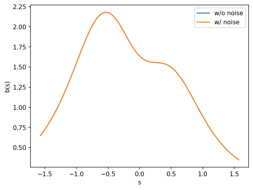
The measured data \(b\) contain both white noise \(\bar{b}\) and truly converted \(b_0\) from \(Ax_\text{t}\).

Descritized linear equation is as follows:

\[Ax = b_0 + \bar{b} = b\]

The noise variance is \(1.0 \times 10^{-4}\).

b_0 = A.dot(x_t)
rng = np.random.default_rng()
b_noise = rng.normal(0, 1.0e-4, b_0.size)
b = b_0 + b_noise

In term of regularization, let us think tikhonov regularization, that is, \(L = I\) and \(x_0 = 0\). And as an optimization method, let us use L-curve method as described above. Lcurve is defined in cherab.phix.inversion module.

lcurve = Lcurve(sigma, u, vh.T, data=b)

Let us solve the inverse problem.

bounds = (-20.0, 2.0)  # bounds of log10 of regularization parameter
sol, status = lcurve.solve(bounds=bounds, disp=False)
print(status)

                    message: ['requested number of basinhopping iterations completed successfully']
                    success: True
                        fun: -373.25031303000344
                          x: [-8.201e+00]
                        nit: 100
      minimization_failures: 0
                       nfev: 2550
                       njev: 1275
 lowest_optimization_result:  message: CONVERGENCE: REL_REDUCTION_OF_F_<=_FACTR*EPSMCH
                              success: True
                               status: 0
                                  fun: -373.25031303000344
                                    x: [-8.201e+00]
                                  nit: 4
                                  jac: [ 6.168e-03]
                                 nfev: 16
                                 njev: 8
                             hess_inv: <1x1 LbfgsInvHessProduct with dtype=float64>

Plot measured data w/ or w/o noise

The noise level is so mute that there is no clear difference between those. However this causes to arise the ill-posed problem due to the kernel function.

plt.plot(s, b_0)
plt.plot(s, b)
plt.legend(["w/o noise", "w/ noise"])
plt.xlabel("s")
plt.ylabel("b(s)");

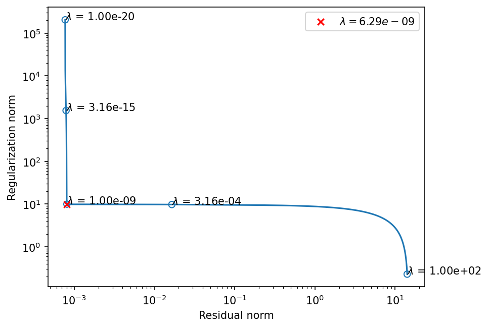
Plot L-curve

lcurve.plot_L_curve(bounds=bounds, n_beta=500, scatter_plot=5, scatter_annotate=True)

(<Figure size 960x720 with 1 Axes>,
 <AxesSubplot:xlabel='Residual norm', ylabel='Regularization norm'>)

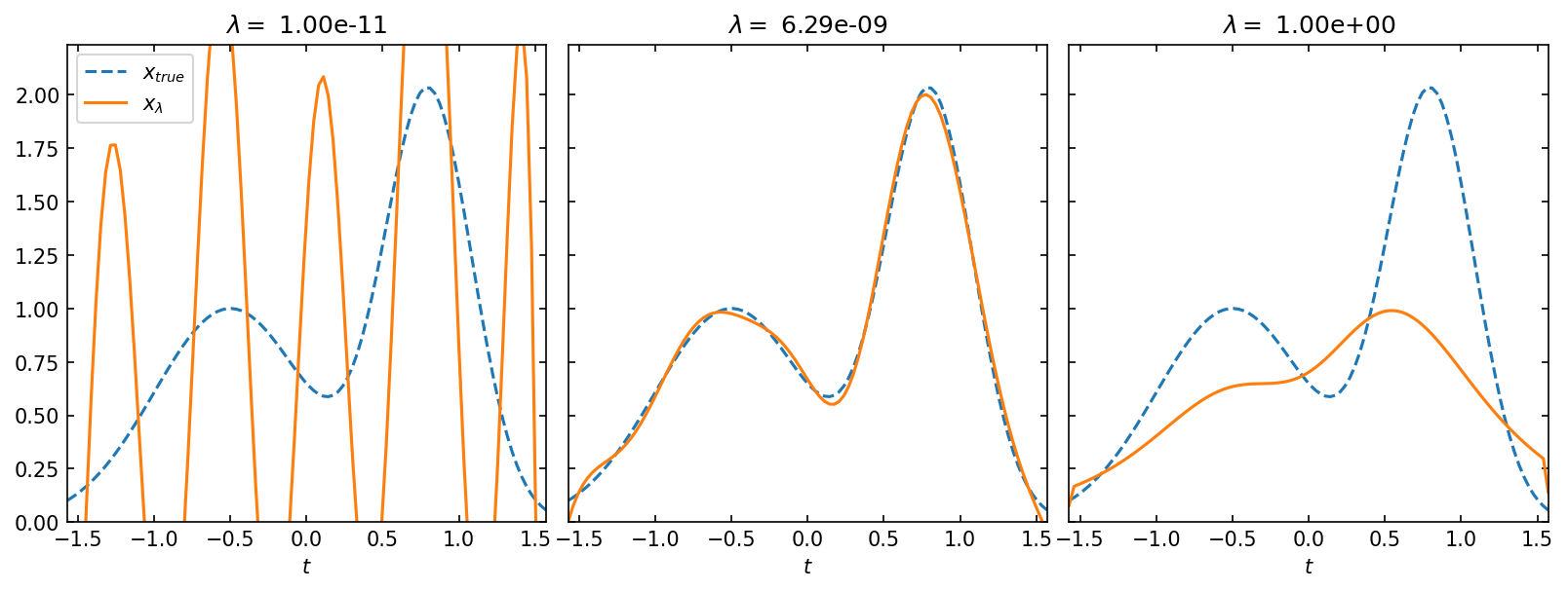
Compare true solution \(x_\text{t}\) with estimated \(x_\lambda\)

Varing regularization parameters makes the interestingly difference between the true solution with estimated one.

Here, let us compare the solutions varied from \(\lambda=10^{-11}, \lambda_\text{opt}, 1.0\). (\(\lambda_\text{opt}\) is the optimized regularization parameter.)

lambdas = [1.0e-11, lcurve.lambda_opt, 1.0]

fig, axes = plt.subplots(1, 3, figsize=(10, 3))
fig.tight_layout(pad=-2.0)
labels = [f"$\\lambda =$ {i:.2e}" for i in lambdas]
i = 0
for ax, beta, label in zip(axes, lambdas, labels):
    ax.plot(t, x_t, "--", label="$x_{true}$")
    ax.plot(t, lcurve.inverted_solution(beta=beta), label="$x_\\lambda$")

    ax.set_xlim(t.min(), t.max())
    ax.set_ylim(0, x_t.max() * 1.1)
    ax.set_xlabel("$t$")
    ax.set_title(label)
    ax.tick_params(direction="in", labelsize=10, which="both", top=True, right=True)
    if i < 1:
        ax.legend()
    else:
        ax.set_yticklabels([])
    i += 1

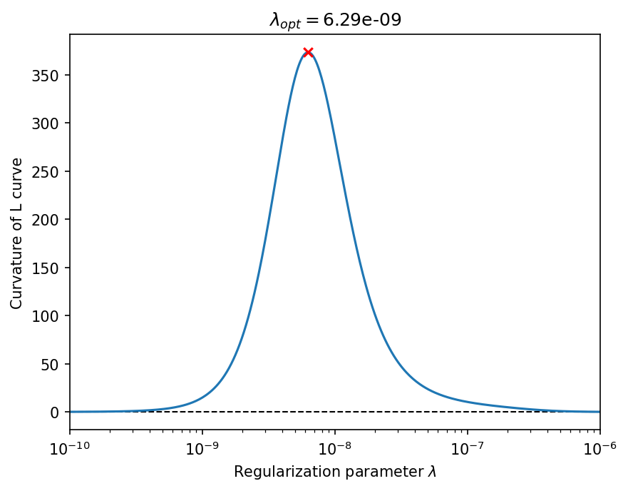
plot L-curve curvature

_, ax = lcurve.plot_curvature(bounds=(-10, -6), n_beta=500)
ax.set_title("$\\lambda_{} = ${:.2e}".format("{opt}", lcurve.lambda_opt));

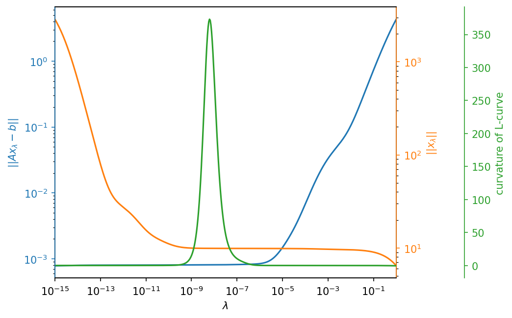
Plot \(\|Ax_\lambda - b\|\), \(\|x_\lambda\|\), and curvature

fig, ax1 = plt.subplots(dpi=150)
fig.subplots_adjust(right=0.85)

ax2 = ax1.twinx()
ax3 = ax1.twinx()

ax3.spines.right.set_position(("axes", 1.2))

# calculation of the values
lambdas = np.logspace(-15, 0, num=500)
rhos = [lcurve.residual_norm(beta) for beta in lambdas]
etas = [lcurve.regularization_norm(beta) for beta in lambdas]
kappa = [lcurve.curvature(beta) for beta in lambdas]

# plot lines
(p1,) = ax1.loglog(lambdas, rhos, color="C0")
(p2,) = ax2.loglog(lambdas, etas, color="C1")
(p3,) = ax3.semilogx(lambdas, kappa, color="C2")

# set axes properties
ax1.set(xlim=(lambdas[0], lambdas[-1]), xlabel=r"$\lambda$", ylabel=r"$||Ax_\lambda - b||$")
ax2.set(ylabel=r"$||x_\lambda||$")
ax3.set(ylabel="curvature of L-curve")

ax1.yaxis.label.set_color(p1.get_color())
ax2.yaxis.label.set_color(p2.get_color())
ax3.yaxis.label.set_color(p3.get_color())

ax1.tick_params(axis="y", colors=p1.get_color())
ax2.tick_params(axis="y", colors=p2.get_color())
ax3.tick_params(axis="y", colors=p3.get_color())

ax3.spines["left"].set_color(p1.get_color())
ax2.spines["right"].set_color(p2.get_color())
ax3.spines["right"].set_color(p3.get_color())

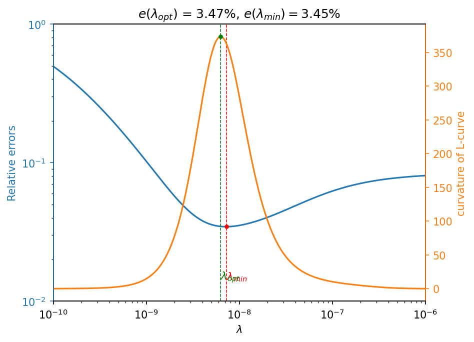
check the error of solutions

The relative error is defined as follows:

\[e(\lambda) = \frac{||x_\text{t} - x_\lambda||}{||x_\text{t}||}.\]

def error(values, true):
    return np.linalg.norm(true - values) / np.linalg.norm(true)


# set regularization parameters
lambdas = np.logspace(-10, -6, num=500)

# calculate errors
errors = np.asarray([error(lcurve.inverted_solution(beta), x_t) for beta in lambdas])
lambda_min = lambdas[errors.argmin()]
error_min = errors.min()
error_opt = error(sol, x_t)

# calculate curvatures
kappa = np.asarray([lcurve.curvature(beta) for beta in lambdas])

# create figure
fig, ax1 = plt.subplots(dpi=150)
ax2 = ax1.twinx()

# plot errors and curvatures
(p1,) = ax1.loglog(lambdas, errors, color="C0")
(p2,) = ax2.semilogx(lambdas, kappa, color="C1")

# plot minimum error vertical line and point
ax1.vlines(lambda_min, 0.01, 1, color="r", linestyle="--", linewidth=0.75)
ax1.scatter(lambda_min, error_min, color="r", marker="o", s=10, zorder=2)
ax1.text(
    lambda_min,
    1.5e-2,
    "$\\lambda_{min}$",
    color="r",
    horizontalalignment="left",
    verticalalignment="center",
)

# plot maximum curvature vertical line and point
ax1.vlines(lcurve.lambda_opt, 0.01, 1, color="g", linestyle="--", linewidth=0.75)
ax2.scatter(lcurve.lambda_opt, lcurve.curvature(lcurve.lambda_opt), color="g", marker="o", s=10, zorder=2)
ax1.text(
    lcurve.lambda_opt,
    1.5e-2,
    "$\\lambda_{opt}$",
    color="g",
    horizontalalignment="left",
    verticalalignment="center",
)

# set axes
ax1.set(
    xlim=(lambdas[0], lambdas[-1]), ylim=(0.01, 1), xlabel=r"$\lambda$", ylabel="Relative errors"
)
ax2.set(ylabel="curvature of L-curve")

ax1.yaxis.label.set_color(p1.get_color())
ax2.yaxis.label.set_color(p2.get_color())

ax1.tick_params(axis="y", colors=p1.get_color())
ax2.tick_params(axis="y", colors=p2.get_color())

ax2.spines["left"].set_color(p1.get_color())
ax2.spines["right"].set_color(p2.get_color())

ax1.set_title(
    "$e(\\lambda_{})$ = {:.2%}, $e(\\lambda_{}) = ${:.2%}".format(
        "{opt}", error_opt, "{min}", error_min
    )
);

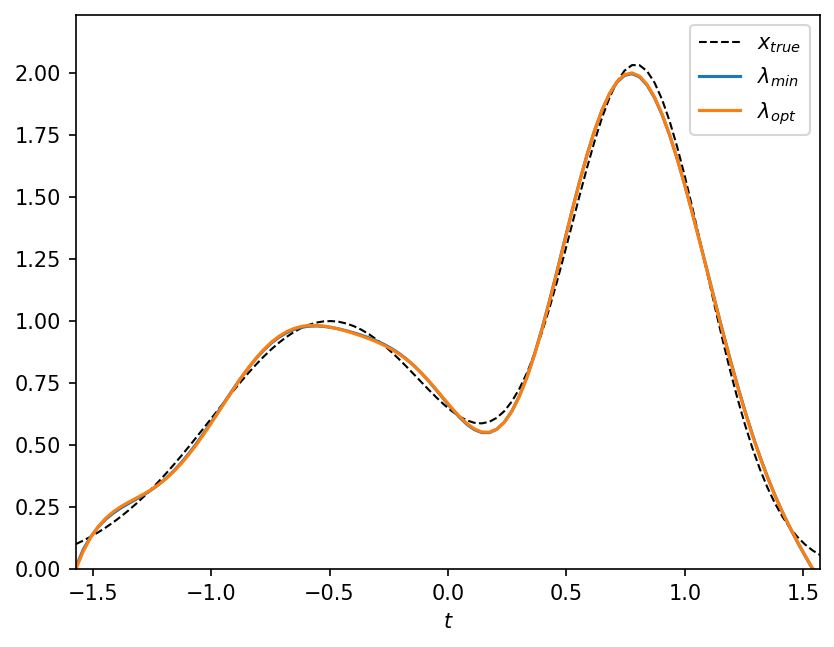
Compare minimum error solution with Lcurve-optimized \(x_\lambda\) one

fig, ax = plt.subplots()
ax.plot(t, x_t, "k--", label="$x_{true}$", linewidth=1.0)
ax.plot(t, lcurve.inverted_solution(lambda_min), label="$\\lambda_{min}$")
ax.plot(t, sol, label="$\\lambda_{opt}$")
ax.set_xlabel("$t$")
ax.set_xlim(t.min(), t.max())
ax.set_ylim(0, x_t.max() * 1.1)
ax.legend()

<matplotlib.legend.Legend at 0x7f6ca9645940>

---

GCV criterion

Diffinition

Generalized Cross-Validation’s idea is that the best modell for the measurements is the one that best predicts each measurement as a function of the others. The GCV estimate of \(\lambda\) is chosen as follows:

\[\begin{split}\begin{align} \lambda_\text{opt} &:= \arg \min_{\lambda} GCV(\lambda)\\ GCV(\lambda) &:= \frac{\rho(\lambda)}{|1 - \text{tr}{T(\lambda)}|^2}, \end{align}\end{split}\]

where

\[\begin{split}\begin{align} \rho(\lambda) &:= ||Ax_\lambda - b||^2\\ T(\lambda)b &:= Ax_\lambda. \end{align}\end{split}\]

Using SVD components, \(GCV(\lambda)\) is replaced as follows:

\[GCV(\lambda) = \frac{\rho(\lambda)}{\left[1 - \sum_{i=1}^r w_i(\lambda) \right]^2}.\]

from cherab.phix.inversion import GCV

gcv = GCV(sigma, u, vh.T, data=b)

bounds = (-20.0, 2.0)  # bounds of log10 of regularization parameter
sol, status = gcv.solve(bounds=bounds, disp=False)
print(status)

                    message: ['requested number of basinhopping iterations completed successfully']
                    success: True
                        fun: 2.68607600493509e-09
                          x: [-2.000e+01]
                        nit: 100
      minimization_failures: 0
                       nfev: 310
                       njev: 155
 lowest_optimization_result:  message: CONVERGENCE: NORM_OF_PROJECTED_GRADIENT_<=_PGTOL
                              success: True
                               status: 0
                                  fun: 2.68607600493509e-09
                                    x: [-2.000e+01]
                                  nit: 1
                                  jac: [ 1.118e-10]
                                 nfev: 4
                                 njev: 2
                             hess_inv: <1x1 LbfgsInvHessProduct with dtype=float64>

Plot error function and GCV

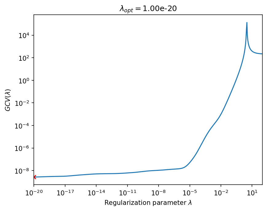
The results of the GCV optimization shows that GCV does not work for this inversion problem.

_, ax = gcv.plot_gcv(bounds=bounds, n_beta=500)
ax.set_title("$\\lambda_{} = ${:.2e}".format("{opt}", gcv.lambda_opt));