Note
This page was generated from docs/notebooks/plasma/plasma_parameters.ipynb.
Typical plasma parameters#
Using the experimental result measured by the langmuir probe, electron density and temperature has been specified at 2 points. Considering both experimental and equilibrium data calculated by TSC (Tokamak Simulation Code) has enabled us to obtain their 2-D profiles.
[1]:
import numpy as np
from matplotlib import pyplot as plt
from matplotlib.ticker import ScalarFormatter
from raysect.optical import World

from cherab.core.math import sample3d
from cherab.phix.plasma import import_plasma
from cherab.phix.plasma.species import PHiXSpecies
from cherab.phix.tools.raytransfer import import_phix_rtc
from cherab.phix.tools.visualize import show_phix_profiles

plt.rcParams["figure.dpi"] = 150
world = World()
plasma, eq = import_plasma(world)
species = PHiXSpecies(equilibrium=eq)
rtc = import_phix_rtc(world, equilibrium=eq)
loading plasma (data from: phix10)...
[2]:
dr = rtc.material.dr
dz = rtc.material.dz
nr = rtc.material.grid_shape[0]
nz = rtc.material.grid_shape[2]
rmin = rtc.material.rmin
zmin = rtc.transform[2, 3]
rmax = rmin + dr * nr
zmax = zmin + dz * nz
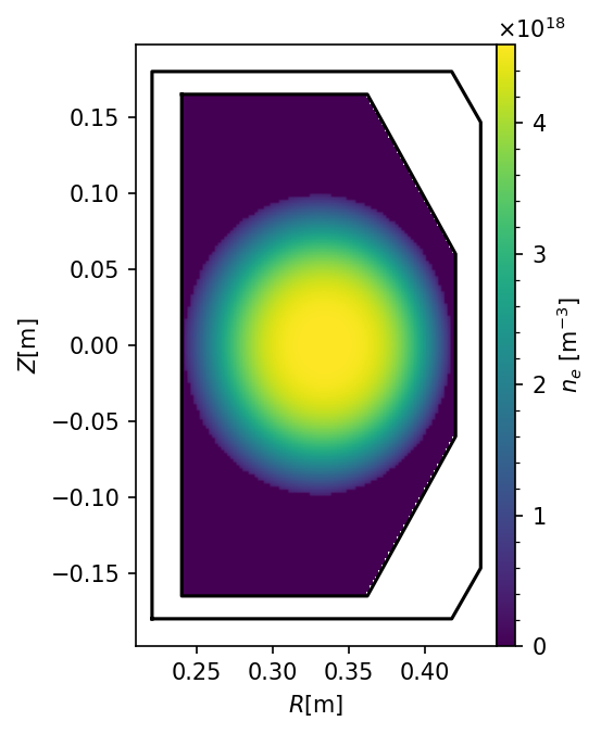
Plotting the plasma parameters distribution in 1D vs \(\psi_\text{normalized}\) and 2D \(r-z\) space#
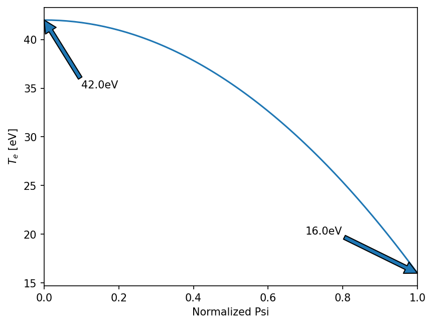
Plasma parameters (\(n_\text{e}, T_\text{e}\)) is assumed to distribute as quadratic function along to \(\psi\). For instance, \(n_\text{e}\) represents as follows:
\[n_e = (n_{\min} - n_{\max}) \psi^2 + n_{\min}\]
The values of \(n_{\min}\) and \(n_{\max}\) are used as an experimental data measured by the langmuir probe which locates both near magnetic axis and LCFS.
[3]:
x = np.linspace(0, 1, 100)
y = [species.temp1d(i) for i in x]
plt.plot(x, y)
plt.xlabel("Normalized Psi")
plt.ylabel("$T_e$ [eV]")
plt.xlim([0, 1])
plt.annotate(f"{y[0]}eV", (x[0], y[0]), (0.1, 35), arrowprops=dict())
plt.annotate(f"{y[-1]}eV", (x[-1], y[-1]), (0.7, 20), arrowprops=dict());
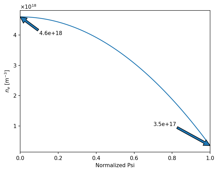
[4]:
x = np.linspace(0, 1, 100)
y = [species.dens1d(i) for i in x]
fig, ax = plt.subplots()
ax.plot(x, y)
ax.yaxis.set_major_formatter(ScalarFormatter(useMathText=True))
ax.set_xlabel("Normalized Psi")
ax.set_ylabel("$n_e$ [m$^{-3}$]")
ax.set_xlim([0, 1])
plt.annotate(f"{y[0]}", (x[0], y[0]), (0.1, 4e18), arrowprops=dict())
plt.annotate(f"{y[-1]}", (x[-1], y[-1]), (0.7, 1e18), arrowprops=dict());
[5]:
r, _, z, ne_samples = sample3d(
    plasma.electron_distribution.density, (rmin, rmax, nr), (0, 0, 1), (zmin, zmax, nz)
)
show_phix_profiles(
    ne_samples.squeeze(),
    clabel="$n_e$ [m$^{-3}$]",
    cmap="viridis",
    scientific_notation=True,
    rtc=rtc,
);
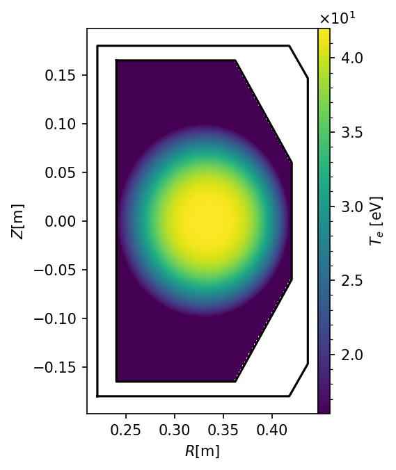
[6]:
r, _, z, te_samples = sample3d(
    plasma.electron_distribution.effective_temperature,
    (rmin, rmax, nr),
    (0, 0, 1),
    (zmin, zmax, nz),
)
show_phix_profiles(te_samples.squeeze(), clabel="$T_e$ [eV]", cmap="viridis", rtc=rtc);
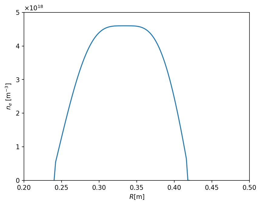
Density Profile along R axis on the equatorial plane.#
[7]:
r, _, z, t_samples = sample3d(
    plasma.electron_distribution.density,
    (rmin, rmax, nr),
    (0, 0, 1),
    (eq.magnetic_axis.y, eq.magnetic_axis.y, 1),
)
fig, ax = plt.subplots()
ax.plot(r, t_samples.ravel())
ax.yaxis.set_major_formatter(ScalarFormatter(useMathText=True))
plt.xlabel("$R$[m]")
plt.ylabel("$n_e$ [m$^{-3}$]")
plt.xlim([0.2, 0.5])
plt.ylim([0, 5e18]);
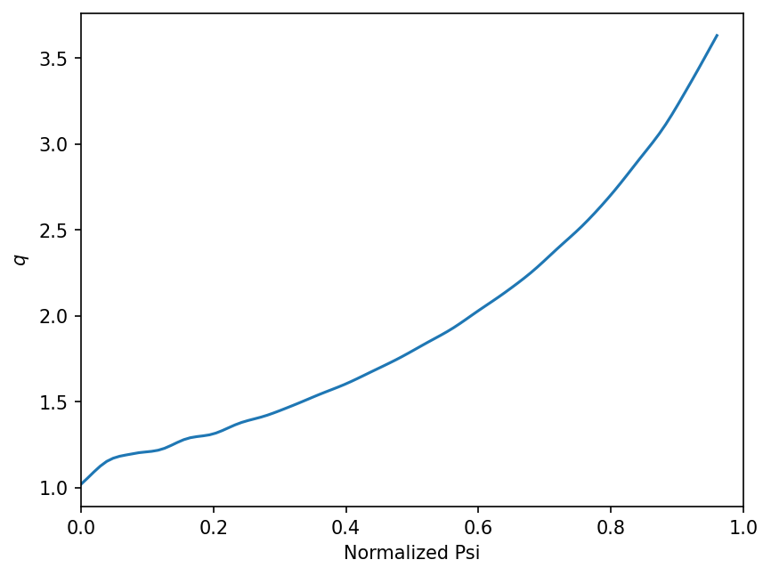
Q profile as a function of \(\psi_\text{normalized}\)#
[8]:
x = np.linspace(0, 0.96, 100)
y = [eq.q(i) for i in x]
plt.plot(x, y)
plt.xlabel("Normalized Psi")
plt.ylabel("$q$")
plt.xlim([0, 1]);