Note

This page was generated from docs/notebooks/inversion/RTM_analysis.ipynb.

Analysis of RTM using SVD method

According to the theorem of tomographic inversion, the inversion solution \(x_\lambda\) with the regularization term and the singular value decomposition is represented as follows:

\[x_\lambda = \sum_{i=1}^r w_i(\lambda) \frac{u_i^\mathsf{T}b}{\sigma_i}L^{-1}v_i.\]

Here, let us look into the SVD elements and consider what role each of them plays.

from pathlib import Path

import numpy as np
from matplotlib import pyplot as plt
from matplotlib.colors import CenteredNorm
from mpl_toolkits.axes_grid1 import ImageGrid
from numpy.lib.format import open_memmap
from raysect.optical import World

from cherab.phix.tools import profile_1D_to_2D
from cherab.phix.tools.raytransfer import import_phix_rtc

RTM_DIR = Path().cwd().parent.parent.parent / "output" / "RTM" / "2022_12_13_00_49_29"

world = World()
rtc = import_phix_rtc(world)

Compare \(L=\text{Laplacian}\) vs \(L=I\)

Let us see the difference of SVD components between \(L=\text{laplacian}\) and \(L=I\).

Load SVD matrices and values with \(L=\text{Laplacian}\)

u = open_memmap(RTM_DIR / "w_laplacian" / "u.npy")
s = open_memmap(RTM_DIR / "w_laplacian" / "s.npy")
vh = open_memmap(RTM_DIR / "w_laplacian" / "vh.npy")
L_inv_V = open_memmap(RTM_DIR / "w_laplacian" / "L_inv_V.npy")

Load SVD matrices and values without Laplacian i.e. \(L=I\)

u_w = open_memmap(RTM_DIR / "wo_laplacian" / "u.npy")
s_w = open_memmap(RTM_DIR / "wo_laplacian" / "s.npy")
vh_w = open_memmap(RTM_DIR / "wo_laplacian" / "vh.npy")

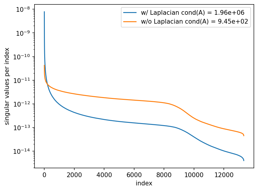
Singular values: \(\sigma_i\)

fig, ax = plt.subplots(dpi=150)
ax.semilogy(s, label=f"w/ Laplacian cond(A) = {s.max() / s.min():.2e}")
ax.semilogy(s_w, label=f"w/o Laplacian cond(A) = {s_w.max() / s_w.min():.2e}")
ax.set_xlabel("index")
ax.set_ylabel("singular values per index")
ax.legend();

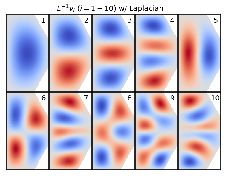
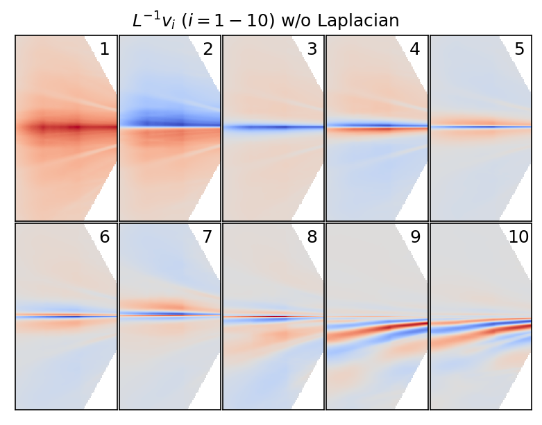
Basis vector: \(L^{-1}v_i\)

These vectors play an important role with tomographic reconstruction because the inverse solution consists of the series of vector \(L^{-1}v_i\), which is regarded as a basis vector of the solution.

fig = plt.figure(dpi=150)
grid = ImageGrid(fig, 111, (2, 5))
for i in range(10):
    masked_profile2d = np.ma.masked_array(
        profile_1D_to_2D(L_inv_V[:, i], rtc), mask=np.logical_not(rtc.mask.squeeze())
    ).T
    grid[i].imshow(masked_profile2d, cmap="coolwarm", norm=CenteredNorm())
    grid[i].text(78, 5, f"{i+1}", fontsize=12, color="k", va="top", ha="center")
    grid[i].set_xticks([])
    grid[i].set_yticks([])

fig.suptitle("$L^{-1}v_i\\ (i=1-10)$ w/ Laplacian", y=0.92);

fig = plt.figure(dpi=150)
grid = ImageGrid(fig, 111, (2, 5))
for i in range(10):
    masked_profile2d = np.ma.masked_array(
        profile_1D_to_2D(vh_w[i, :], rtc), mask=np.logical_not(rtc.mask.squeeze())
    ).T
    grid[i].imshow(masked_profile2d, cmap="coolwarm", norm=CenteredNorm())
    grid[i].text(78, 5, f"{i+1}", fontsize=12, color="k", va="top", ha="center")
    grid[i].set_xticks([])
    grid[i].set_yticks([])

fig.suptitle("$L^{-1}v_i\\ (i=1-10)$ w/o Laplacian", y=0.92);

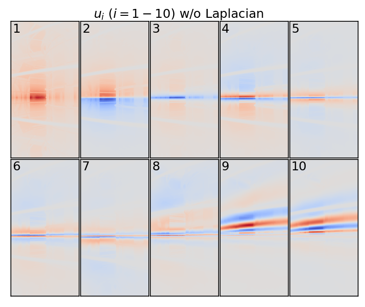
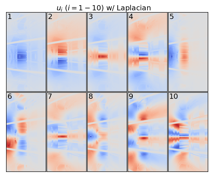
Left-singular vectors: \(u_i\)

These vectors are related to the measured camera images. We can find the Laplacian effect in them as well.

fig = plt.figure(dpi=150)
grid = ImageGrid(fig, 111, (2, 5))
for i in range(10):
    grid[i].imshow(u[:, i].reshape((256, 512)).T, cmap="coolwarm", norm=CenteredNorm())
    grid[i].text(5, 5, f"{i+1}", fontsize=12, color="k", va="top")
    grid[i].set_xticks([])
    grid[i].set_yticks([])

fig.suptitle("$u_i\\ (i=1-10)$ w/ Laplacian", y=0.92);

fig = plt.figure(dpi=150)
grid = ImageGrid(fig, 111, (2, 5))
for i in range(10):
    grid[i].imshow(u_w[:, i].reshape((256, 512)).T, cmap="coolwarm", norm=CenteredNorm())
    grid[i].text(5, 5, f"{i+1}", fontsize=12, color="k", va="top")
    grid[i].set_xticks([])
    grid[i].set_yticks([])

fig.suptitle("$u_i\\ (i=1-10)$ w/o Laplacian", y=0.92);