Note
This page was generated from docs/notebooks/observer/fast_camera_raytracing.ipynb.
Ray-tracing simulation of fast camera#
[ ]:
import numpy as np
from matplotlib import pyplot as plt
from mpl_toolkits.axes_grid1 import ImageGrid
from raysect.optical import World
from raysect.optical.observer import PowerPipeline2D, RGBAdaptiveSampler2D, RGBPipeline2D

from cherab.phix.machine import import_phix_mesh
from cherab.phix.observer import import_phix_camera
from cherab.phix.plasma import import_plasma
Create scene graph#
[ ]:
# scene world
world = World()

# import plasma
plasma, eq = import_plasma(world)

# import phix mesh
mesh = import_phix_mesh(world, reflection=True)

# import phix camera
camera = import_phix_camera(world)
Set up pipelines#
[ ]:
# RGB image and Power pipelines
# NOTE: if you excute the code in .py script, the progress image can be displayed
# when `display_progress = True`.
rgb = RGBPipeline2D(display_unsaturated_fraction=1.0, name="sRGB", display_progress=False)
power = PowerPipeline2D(display_progress=False, name="power")

# set camera's pipeline property
camera.pipelines = [rgb, power]
Set other camera parameters#
[ ]:
# set sampler
sampler = RGBAdaptiveSampler2D(rgb, ratio=10, fraction=0.2, min_samples=10, cutoff=0.05)

camera.frame_sampler = sampler
camera.min_wavelength = 400
camera.max_wavelength = 780
camera.spectral_rays = 1
camera.spectral_bins = 20  # spectrum resolution between 400 - 780 nm in wavelength
camera.per_pixel_samples = 10
camera.lens_samples = 10
Execute Ray-tracing#
[ ]:
plt.ion()
camera.observe()
Save images and power data#
[ ]:
Ray-traced images are shown below:
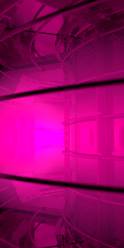
RGB image#
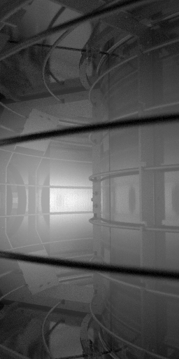
Power monochrome image#
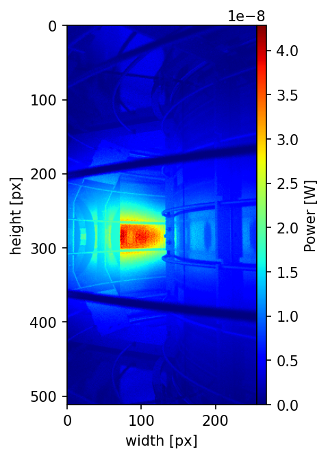
Show calculated power distribution#
[ ]:
fig = plt.figure(dpi=150)
grids = ImageGrid(fig, 111, (1, 1), axes_pad=0, cbar_mode="each")
mappable = grids[0].imshow(power.frame.mean.T, cmap="jet")
grids[0].set_xlabel("width [px]")
grids[0].set_ylabel("height [px]")
cbar = plt.colorbar(mappable, cax=grids.cbar_axes[0])
cbar.set_label("Power [W]")
Note
demos/synthetic_calculation.py is the script file having the same workflow as the above codes.