Note

This page was generated from docs/notebooks/others/derivative_operator.ipynb.

Derivative Operator

Here, we show you what the derivative operator and how it works on the example images

Filtering in an image means to perform some kind of processing on a pixel value \(I(x, y)\) using its neighboring pixel values as follows:

\[I'(x, y) = \sum_{i=-1}^{1}\sum_{j=-1}^{1}K(i, j)I(x + i, y + j),\]

where, \(I'(x, y)\): performed pixel value, \(K\): kernel matrix.

The first derivative operator in each direction (\(x\), \(y\)) is represented as following kernels:

\[\begin{split}K_x = \begin{bmatrix} 0 & 0 & 0 \\ -1 & 1 & 0 \\ 0 & 0 & 0 \end{bmatrix}, \quad K_y = \begin{bmatrix} 0 & -1 & 0 \\ 0 & 1 & 0 \\ 0 & 0 & 0 \end{bmatrix}.\end{split}\]

Laplacian Operator is a also derivative operator which is used to find edges in an image and represented as following kernels:

\[\begin{split}K_4 = \begin{bmatrix} 0 & 1 & 0\\ 1 & -4 & 1\\ 0 & 1 & 0 \end{bmatrix}, \quad K_8 = \begin{bmatrix} 1 & 1 & 1\\ 1 & -8 & 1\\ 1 & 1 & 1 \end{bmatrix},\end{split}\]

where \(K_4\): a kernel that considers the contribution of 4 nearest neighbors (top, bottom, left, right) to the pixel of interest, \(K_8\): a kernel that considers 8 nearest neighbors (top, bottom, left, right, diagonal) to the pixel of interest.

To perform these operator to a image converted 1-D vector array, we generate derivative matrices.

import numpy as np
from matplotlib import pyplot as plt
from matplotlib.cbook import get_sample_data
from matplotlib.colors import CenteredNorm
from mpl_toolkits.axes_grid1 import ImageGrid
from PIL import Image

from cherab.phix.tools import compute_dmat

Visualize derivative matrix

Try to create the simple derivative matrix (10, 10). Firstly, create the mapping array denoting 2-D image shape and the element of which denotes a index.

# mapping array
mapping_array = np.arange(0, 50, dtype=np.int32).reshape(10, 5)

Plot derivative matrix as a sparse matrix and compare \(K_x\) and \(K_4\) kernel

fig, axes = plt.subplots(1, 2, dpi=150, tight_layout=True)
for ax, kernel_type, kernel_name in zip(axes, ["x", "laplacian4"], ["x", "4"]):

    # calculate derivative matrix
    dmat = compute_dmat(mapping_array, kernel_type=kernel_type)

    # plot sparse matrix
    ax.spy(dmat, markersize=2)
    ax.set_title(f"derivative matrix $K_{kernel_name}$", pad=25)

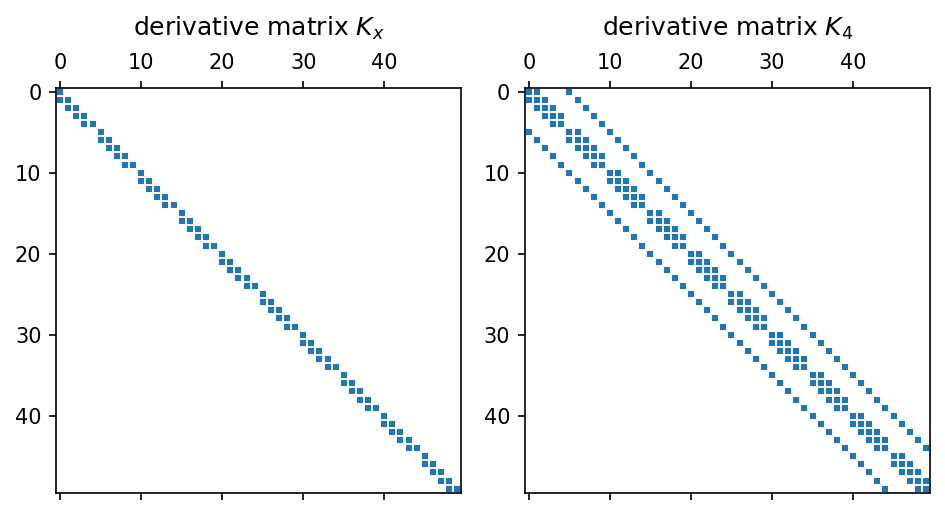
show laplacian matrix \(K_4\) in (10, 10) size as a numpy array.

dmat.toarray()[0:10, 0:10]

array([[-4.,  1.,  0.,  0.,  0.,  1.,  0.,  0.,  0.,  0.],
       [ 1., -4.,  1.,  0.,  0.,  0.,  1.,  0.,  0.,  0.],
       [ 0.,  1., -4.,  1.,  0.,  0.,  0.,  1.,  0.,  0.],
       [ 0.,  0.,  1., -4.,  1.,  0.,  0.,  0.,  1.,  0.],
       [ 0.,  0.,  0.,  1., -4.,  0.,  0.,  0.,  0.,  1.],
       [ 1.,  0.,  0.,  0.,  0., -4.,  1.,  0.,  0.,  0.],
       [ 0.,  1.,  0.,  0.,  0.,  1., -4.,  1.,  0.,  0.],
       [ 0.,  0.,  1.,  0.,  0.,  0.,  1., -4.,  1.,  0.],
       [ 0.,  0.,  0.,  1.,  0.,  0.,  0.,  1., -4.,  1.],
       [ 0.,  0.,  0.,  0.,  1.,  0.,  0.,  0.,  1., -4.]])

Apply the derivative matrix to a sample image

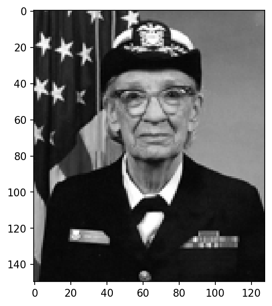
Next, let us to apply derivative matrices to pixels of a sample image.

Load sample image data from the matplotlib library.

with get_sample_data("grace_hopper.jpg") as file:
    arr_image = plt.imread(file)

# resize the image deu to the large size.
with Image.fromarray(arr_image, mode="RGB") as im:
    (width, height) = (im.width // 4, im.height // 4)
    arr_image = np.array(im.resize((width, height)))

# convert RGB image to monotonic one
arr_image = arr_image.mean(axis=2)

# show image
print(f"image array shape: {arr_image.shape}")
fig, ax = plt.subplots(dpi=150)
ax.imshow(arr_image, cmap="gray");

image array shape: (150, 128)

# create mapping array
image_map = np.arange(0, arr_image.size, dtype=np.int32).reshape(arr_image.shape)

# create derivative matrix with Kx
dmatx = compute_dmat(image_map, kernel_type="x")

# create derivative matrix with Ky
dmaty = compute_dmat(image_map, kernel_type="y")

# create laplacian matrix with K8
laplacian_mat = compute_dmat(image_map, kernel_type="laplacian8")

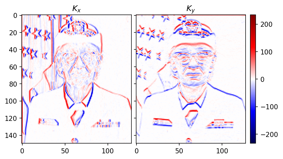
The filtered images are calculated by multiplying the image vector by each derivative matrix.

filtered_x = np.reshape(dmatx @ arr_image.ravel(), arr_image.shape)
filtered_y = np.reshape(dmaty @ arr_image.ravel(), arr_image.shape)
filtered_laplacian = np.reshape(laplacian_mat @ arr_image.ravel(), arr_image.shape)

Compare \(K_x\) and \(K_y\) kernel

# extract max and min value
vmax = max(filtered_x.max(), filtered_y.max())
vmin = min(filtered_x.min(), filtered_y.min())
half_range = max(abs(vmax), abs(vmin))
norm = CenteredNorm(vcenter=0, halfrange=half_range)

# show each image
fig = plt.figure(dpi=150)
grids = ImageGrid(fig, 111, nrows_ncols=(1, 2), axes_pad=0.1, cbar_mode="single")
for ax, filtered_image, title in zip(grids, [filtered_x, filtered_y], ["$K_x$", "$K_y$"]):
    mappable = ax.imshow(filtered_image, cmap="seismic", norm=norm)
    ax.set_title(title)

cbar = plt.colorbar(mappable, cax=grids.cbar_axes[0])

Show the laplacian filtered image \(K_8\)

fig, ax = plt.subplots(dpi=150)
mappable = ax.imshow(filtered_laplacian, cmap="seismic", norm=CenteredNorm())
ax.set_title("$K_8$")
cbar = plt.colorbar(mappable)

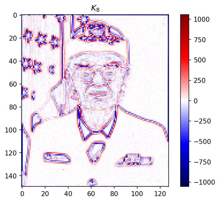
These results show that the edge of the image is emphasized clearly. So, we take advantage of this operator to smooth tomographic reconstructions.