Note
This page was generated from docs/notebooks/plasma/atomic_data_analysis.ipynb.
Typical atomic data used in PHiX#
[1]:
import numpy as np
from matplotlib import pyplot as plt
from raysect.optical import World

from cherab.phix.plasma import import_plasma

plt.rcParams["font.size"] = 14
plt.rcParams["figure.dpi"] = 150
[2]:
world = World()
plasma, eq = import_plasma(world)
loading plasma (data from: phix10)...
The photon emission models used in PHiX are listed as follows:
[3]:
[i for i in plasma.models]
[3]:
[<PlasmaModel - Bremsstrahlung>,
 <ExcitationLine: element=hydrogen, charge=0, transition=(3, 2)>,
 <ExcitationLine: element=hydrogen, charge=0, transition=(4, 2)>,
 <ExcitationLine: element=hydrogen, charge=0, transition=(5, 2)>,
 <ExcitationLine: element=hydrogen, charge=0, transition=(6, 2)>,
 <RecombinationLine: element=hydrogen, charge=0, transition=(3, 2)>,
 <RecombinationLine: element=hydrogen, charge=0, transition=(4, 2)>,
 <RecombinationLine: element=hydrogen, charge=0, transition=(5, 2)>,
 <RecombinationLine: element=hydrogen, charge=0, transition=(6, 2)>]
Species taken into account are listed below as well.
[4]:
species = [i for i in plasma.composition]
print(species)
[<Species: element=hydrogen, charge=0>, <Species: element=hydrogen, charge=1>]
Plotting Photon Emissivity Coefficient (PEC) vs \(T_\text{e}\) for hydrogen transitions#
Plasma emissivity driven by the electron transition from \(j\) to \(i\) : \(\epsilon_{j\rightarrow i}\) [\(\text{W/m}^3\)] is represented by the following expression:
\[\epsilon_{j\rightarrow i} = \sum_\rho \text{PEC}_{\rho, j\rightarrow i}^\text{(exc)}(n_\text{e}, T_\text{e})n_\text{e} n_Z(\rho) + \sum_\nu \text{PEC}_{\nu, j\rightarrow i}^\text{(rec)}(n_\text{e}, T_\text{e})n_\text{e} n_{Z+1}(\nu),\]
where, \(n_\text{e}\): electron density, \(T_\text{e}\): electron temperature, \(n_Z(\rho)\): population number density \(Z\) ions.
[5]:
temp = [10**x for x in np.linspace(np.log10(1), np.log10(1000), num=100)]
dens = [17, 20]  # 10^x [m^-3]

pec_exc = plasma.atomic_data.impact_excitation_pec(species[0].element, species[0].charge, (3, 2))
pec_rem = plasma.atomic_data.recombination_pec(species[0].element, species[0].charge, (3, 2))

fig, ax = plt.subplots(figsize=(8, 6))
ax.loglog(temp, [pec_exc(10 ** dens[0], te) for te in temp], "C0")
ax.loglog(temp, [pec_rem(10 ** dens[0], te) for te in temp], "C1")
ax.loglog(temp, [pec_exc(10 ** dens[1], te) for te in temp], "C0", linestyle="--")
ax.loglog(temp, [pec_rem(10 ** dens[1], te) for te in temp], "C1", linestyle="--")

dens_index1 = str(dens[0])
dens_index2 = str(dens[1])
ax.legend(
    [
        "Excitation $n_e=10^{}$$^{}$ m$^{}$$^{}$".format(dens_index1[0], dens_index1[1], "-", "3"),
        "Recombination $n_e=10^{}$$^{}$ m$^{}$$^{}$".format(
            dens_index1[0], dens_index1[1], "-", "3"
        ),
        "Excitation $n_e=10^{}$$^{}$ m$^{}$$^{}$".format(dens_index2[0], dens_index2[1], "-", "3"),
        "Recombination $n_e=10^{}$$^{}$ m$^{}$$^{}$".format(
            dens_index2[0], dens_index2[1], "-", "3"
        ),
    ]
)

ax.set_title("H$\\alpha$ emission")
ax.set_xlabel("Temperature [eV]")
ax.set_ylabel("PEC [W m$^3$]")
plt.grid(which="both")

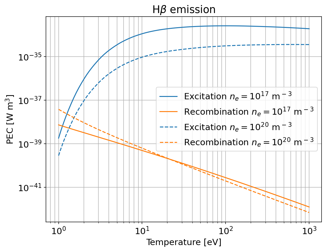
[6]:
pec_exc = plasma.atomic_data.impact_excitation_pec(species[0].element, species[0].charge, (4, 2))
pec_rem = plasma.atomic_data.recombination_pec(species[0].element, species[0].charge, (4, 2))

fig, ax = plt.subplots(figsize=(8, 6))
ax.loglog(temp, [pec_exc(10 ** dens[0], te) for te in temp], "C0")
ax.loglog(temp, [pec_rem(10 ** dens[0], te) for te in temp], "C1")
ax.loglog(temp, [pec_exc(10 ** dens[1], te) for te in temp], "C0", linestyle="--")
ax.loglog(temp, [pec_rem(10 ** dens[1], te) for te in temp], "C1", linestyle="--")

dens_index1 = str(dens[0])
dens_index2 = str(dens[1])
ax.legend(
    [
        "Excitation $n_e=10^{}$$^{}$ m$^{}$$^{}$".format(dens_index1[0], dens_index1[1], "-", "3"),
        "Recombination $n_e=10^{}$$^{}$ m$^{}$$^{}$".format(
            dens_index1[0], dens_index1[1], "-", "3"
        ),
        "Excitation $n_e=10^{}$$^{}$ m$^{}$$^{}$".format(dens_index2[0], dens_index2[1], "-", "3"),
        "Recombination $n_e=10^{}$$^{}$ m$^{}$$^{}$".format(
            dens_index2[0], dens_index2[1], "-", "3"
        ),
    ]
)

ax.set_title("H$\\beta$ emission")
ax.set_xlabel("Temperature [eV]")
ax.set_ylabel("PEC [W m$^3$]")
plt.grid(which="both")