Note

This page was generated from docs/notebooks/inversion/L_curve.ipynb.

L-curve criterion

By P.C. Hansen

Diffinition

Practically, in order to solve inversion problems \(Ax=b\), we need to consider the similar form of least-squeares equations as follows:

\[\begin{split}\begin{align} x_\lambda &= \arg\min\{||Ax - b||_2^2 + \lambda\cdot||L(x - x_0)||_2^2\}\\ & = (A^\mathsf{T}A + \lambda L^\mathsf{T}L)^{-1} (A^\mathsf{T}b + \lambda L^\mathsf{T}x_0). \end{align}\end{split}\]

\(\lambda\) is a real regularization parameter that must be chosen by the user. The vector \(b\) is the given data and the vector \(x_0\) is a priori estimate of \(x\) which is set to zero when no a priori information is available. \(||Ax - b||_2\) is the residual term and \(||L(x - x_0)||_2\) is the regularization term. \(\lambda\) is the parameter which decides the contribution to these terms. And L-curve criterion is the method to balance between these contribution and optmize the inversion solution.

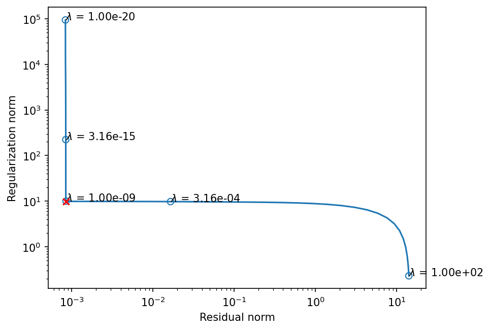
L-curve is precisely following points curve:

\[(||Ax - b||_2, ||L(x - x_0)||_2)\]

L-curve criterion is based on the fact that the optimal reguralization paramter is acheived when the L-curve point:

\[(\log||Ax_\lambda - b||_2,\; \log||L(x_\lambda - x_0)||_2)\]

lies on this corner.

In order to obtain the strict \(\lambda\) on the L-curve “corner” which is defined by the mathmatical method, we can calculate the L-curve carvature \(\kappa\) given by following equation:

\[\begin{split}\begin{align} \kappa &= \frac{f^{\prime\prime}(x)}{\left[1 + f^{\prime}(x)^2\right]^{3/2}}=-2 \eta\rho\frac{\lambda^2 \eta + \lambda \rho + \rho\eta/\eta^\prime}{(\lambda^2 \eta^2 + \rho^2)^{3/2}},\\ \rho &\equiv ||Ax_\lambda - b||_2^2,\\ \eta &\equiv ||L(x_\lambda - x_0)||_2^2,\\ \eta^\prime &\equiv \frac{d\eta}{d\lambda} \end{align}\end{split}\]

Using the singular value decomposion (SVD) fomula, \(x_\lambda\) is described as follows:

\[\begin{split}\begin{align} x_\lambda &= L^{-1}V(\Sigma^\mathsf{T}\Sigma + \lambda I)^{-1}\Sigma^\mathsf{T}\ U^\mathsf{T}b\\ &= L^{-1}V \begin{pmatrix} w_1(\lambda) / \sigma_1 \\ w_2(\lambda) / \sigma_2 \\ \vdots \end{pmatrix} \circ U^\mathsf{T}b\\ &= \sum_{i=1}^K w_i(\lambda) \frac{(u_i, b)}{\sigma_i}L^{-1}v_i, \end{align}\end{split}\]

where,

\[\begin{split}\begin{align} w_i(\lambda) &\equiv \frac{1}{1 + \lambda/\sigma_i^2},\\ U\Sigma V^\mathsf{T} &\equiv (u_1, u_2, ...) \cdot \text{diag}(\sigma_1, \sigma_2,...) \cdot (v_1, v_2, ...)^\mathsf{T} = AL^{-1}. \end{align}\end{split}\]

Here, \(K\equiv\min(M, N)\), which means the size of SVD matrices: \(U=\text{Mat}(M, M)\), \(\Sigma=\text{Mat}(M, N)\), \(V=\text{Mat}(N, N)\), and a priori estimate \(x_0\) is assumed to be 0. Additionally, the symbol \(\circ\) means the Hadamard product.

Also \(\rho, \eta,\) and \(\eta^\prime\) is described by using SVD as follows:

\[\begin{split}\begin{align} \rho &= \sum_{i=1}^K (1 - w_i)^2(u_i, b)^2,\\ \eta &= \sum_{i=1}^K w_i^2 \frac{(u_i, b)^2}{\sigma_i^2},\\ \eta^\prime &= -\frac{2}{\lambda}\sum_{i=1}^K (1 - w_i)w_i^2\frac{(u_i, b)^2}{\sigma_i^2}. \end{align}\end{split}\]

Example ill-posed linear operator equation and applying L-curve criterion into this problem.

As a famouse ill-posed linear equation, Fredholm integral equation is often used:

\[\int_a^b K(s, t) x(t) dt = b(s), \quad c\leq s\leq d.\]

Here, we think the following situation as above equation form:

\[\begin{split}\begin{align} K(s, t) &\equiv (\cos(s) + \cos(t))\left(\frac{\sin(u)}{u}\right)^2,\\ u &\equiv \pi\left(\sin(s) + \sin(t) \right),\\ [a, b] &= [c, d] = \left[-\frac{\pi}{2}, \frac{\pi}{2} \right]. \end{align}\end{split}\]

And, the true solution \(x_\text{t}(t)\) is assumed as follows:

\[x_\text{t}(t) = 2.0 \exp\left[-6(t-0.8)^2 \right] + \exp\left[-2(t+0.5)^2 \right]\]

let us define these function as follows:

import numpy as np
from matplotlib import pyplot as plt

from cherab.phix.inversion import Lcurve

plt.rcParams["figure.dpi"] = 150


def kernel(s: np.ndarray, t: np.ndarray):
    """Kernel of Fredholm integral equation of the first kind."""
    u = np.pi * (np.sin(s) + np.sin(t))
    if u == 0:
        return np.cos(s) + np.cos(t)
    else:
        return (np.cos(s) + np.cos(t)) * (np.sin(u) / u) ** 2


# true solution
def x_t_func(t):
    return 2.0 * np.exp(-6.0 * (t - 0.8) ** 2) + np.exp(-2.0 * (t + 0.5) ** 2)

Let’s descritize the above integral equation. \(s\) and \(t\) are devided to 100 points at even intervals. \(x\) is a 1D vector data \((100, )\) and \(A\) is a \(100\times 100\) matrix. \(A\) is defined using karnel function. When discretizing the integral, the trapezoidal approximation is applied.

# set valiables
s = np.linspace(-np.pi * 0.5, np.pi * 0.5, num=100)
t = np.linspace(-np.pi * 0.5, np.pi * 0.5, num=100)
x_t = x_t_func(t)

# Operater matrix: A
A = np.zeros((s.size, t.size))
A = np.array([[kernel(i, j) for j in t] for i in s])

# trapezoidal rule
A[:, 0] *= 0.5
A[:, -1] *= 0.5
A *= t[1] - t[0]

# simpson rule  -- option
# A[:, 1:-1:2] *= 4.0
# A[:, 2:-2:2] *= 2.0
# A *= (t[1] - t[0]) / 3.0

print(f"condition number of A is {np.linalg.cond(A)}")

condition number of A is 1.3162238461768632e+19

Then excute singular value decomposition of \(A\)

# SVD using the numpy module
u, sigma, vh = np.linalg.svd(A, full_matrices=False)

The measured data \(b\) is added white noise \(\bar{b}\), and truly converted \(b_0\) is computed from \(Ax_\text{t}\).

Descritized linear equation is as follows:

\[Ax = b_0 + \bar{b} = b\]

The noise variance is \(1.0 \times 10^{-4}\).

b_0 = A.dot(x_t)
rng = np.random.default_rng()
b_noise = rng.normal(0, 1.0e-4, b_0.size)
b = b_0 + b_noise

In term of regularization, let us think tikhonov regularization, that is, \(L = I\) and \(x_0 = 0\). And as an optimization method of regulariation parameters, use L-curve method as described above. Lcurve is defined in cherab.phix.inversion module.

lcurv = Lcurve(sigma, u, vh, b)
lcurv.lambdas = 10 ** np.linspace(-20, 2, 100)
lcurv.optimize(10)  # iteration times to find the maximum carvature

completed the optimization (iteration times : 10)

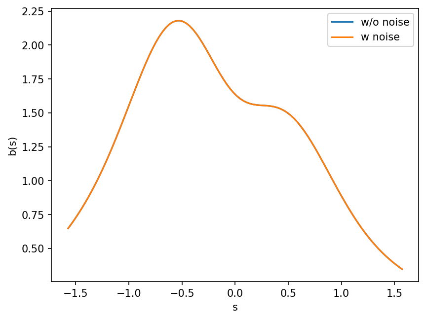
Plot measured data w or w/o noise

The noise level is so mute that there is no clear difference between those. However this causes to arise the ill-posed problem due to the kernel function.

plt.plot(s, b_0)
plt.plot(s, b)
plt.legend(["w/o noise", "w noise"])
plt.xlabel("s")
plt.ylabel("b(s)");

Plot L-curve

lcurv.plot_L_curve(scatter_plot=5, scatter_annotate=True);

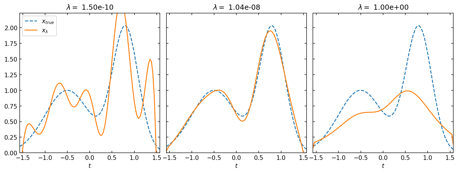
Compare true solution \(x_\text{t}\) with estimated \(x_\lambda\)

Varing regularization parameters makes the interestingly difference between the true solution with estimated one.

Here, let us compare the solutions varied from \(\lambda=10^{-11}, \lambda_\text{opt}, 1.0\). (\(\lambda_\text{opt}\) is the optimized regularization parameter.)

lambdas = [1.5e-10, lcurv.lambda_opt, 1.0]

fig, axes = plt.subplots(1, 3, figsize=(10, 3))
fig.tight_layout(pad=-2.0)
labels = [f"$\\lambda =$ {i:.2e}" for i in lambdas]
i = 0
for ax, beta, label in zip(axes, lambdas, labels):
    ax.plot(t, x_t, "--", label="$x_{true}$")
    ax.plot(t, lcurv.inverted_solution(beta=beta), label="$x_\\lambda$")

    ax.set_xlim(t.min(), t.max())
    ax.set_ylim(0, x_t.max() * 1.1)
    ax.set_xlabel("$t$")
    ax.set_title(label)
    ax.tick_params(direction="in", labelsize=10, which="both", top=True, right=True)
    if i < 1:
        ax.legend()
    else:
        ax.set_yticklabels([])
    i += 1

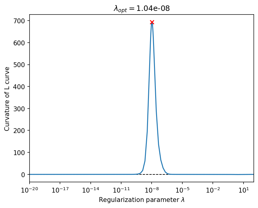
plot L-curve curvature

_, ax = lcurv.plot_curvature()
ax.set_title("$\\lambda_{} = ${:.2e}".format("{opt}", lcurv.lambda_opt));

check the error of solutions

The relative error is defined as follows:

\[e(\lambda) = \frac{||x_\text{t} - x_\lambda||}{||x_\text{t}||}.\]

def error(values, true):
    return np.linalg.norm(true - values) / np.linalg.norm(true)


errors = np.asarray([error(lcurv.inverted_solution(beta), x_t) for beta in lcurv.lambdas])
lambda_min = lcurv.lambdas[errors.argmin()]
error_min = errors.min()
error_opt = errors[np.where(lcurv.lambdas == lcurv.lambda_opt)[0][0]]

# xlim, ylim
xlim = 1.0e-13, 1.0e2
ylim = 1.0e-02, 2.0e2

fig, ax = plt.subplots()

# relative errors
ax.loglog(lcurv.lambdas, errors, color="C0")
ax.text(lcurv.lambdas[35], errors[33], "$e(\\lambda)$", color="C0")

# residual norms
residuals = [lcurv.residual_norm(beta) for beta in lcurv.lambdas]
ax.loglog(lcurv.lambdas, residuals, color="C1")
ax.text(
    lcurv.lambdas[-5], residuals[-1], "$||Ax_\\lambda-b||$", color="C1", horizontalalignment="right"
)

# regularization norms
reguls = [lcurv.regularization_norm(beta) for beta in lcurv.lambdas]
ax.loglog(lcurv.lambdas, reguls, color="C2")
ax.text(lcurv.lambdas[35], reguls[33], "$||Lx_\\lambda||$", color="C2")

# scattered point
min_sol = ax.scatter(lambda_min, error_min, marker="x", color="r")
ax.text(
    lambda_min,
    error_min * 0.8,
    "min($e(\\lambda)$)",
    color="r",
    horizontalalignment="left",
    verticalalignment="top",
)
opt = ax.scatter(lcurv.lambda_opt, error_opt, marker="x", color="g")
ax.text(
    lcurv.lambda_opt,
    error_opt * 0.8,
    "$e(\\lambda_{opt})$",
    color="g",
    horizontalalignment="right",
    verticalalignment="top",
)

ax.set_xlim(*xlim)
ax.set_ylim(*ylim)
ax.set_xlabel("$\\lambda$")
ax.set_title(
    "min($e(\\lambda)$) = {:.2%}, $e(\\lambda_{}) = ${:.2%}".format(error_min, "{opt}", error_opt)
);

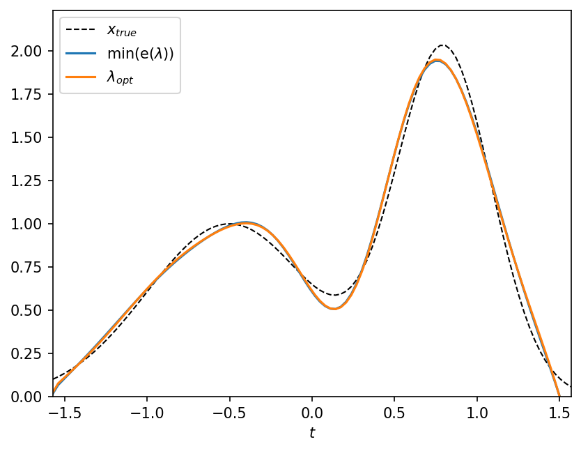
Compare minimum error solution with Lcurve-optimized \(x_\lambda\) one

fig, ax = plt.subplots()
ax.plot(t, x_t, "k--", label="$x_{true}$", linewidth=1.0)
ax.plot(t, lcurv.inverted_solution(beta=lambda_min), label="min(e($\\lambda$))")
ax.plot(t, lcurv.inverted_solution(beta=lcurv.lambda_opt), label="$\\lambda_{opt}$")
ax.set_xlabel("$t$")
ax.set_xlim(t.min(), t.max())
ax.set_ylim(0, x_t.max() * 1.1)
ax.legend();

GCV criterion

Diffinition

Generalized Cross-Validation’s idea is that the best modell for the measurements is the one that best predicts each measurement as a function of the others. The GCV estimate of \(\lambda\) is chosen as follows:

\[\begin{split}\begin{align} \lambda_\text{opt} &:= \arg \min_{\lambda} GCV(\lambda)\\ GCV(\lambda) &:= \frac{\rho(\lambda)}{|1 - \text{tr}{T(\lambda)}|^2}, \end{align}\end{split}\]

where

\[\begin{split}\begin{align} \rho(\lambda) &:= ||Ax_\lambda - b||^2\\ T(\lambda)b &:= Ax_\lambda. \end{align}\end{split}\]

Using SVD components, \(GCV(\lambda)\) is replaced as follows:

\[GCV(\lambda) = \frac{\rho(\lambda)}{\left[1 - \sum_{i=1}^N w_i(\lambda) \right]^2}.\]

from cherab.phix.inversion import GCV

gcv = GCV(sigma, u, vh, b)
gcv.lambdas = 10 ** np.linspace(-20, 2, 100)
gcv.optimize(6)

completed the optimization (iteration times : 6)

Plot error function and GCV

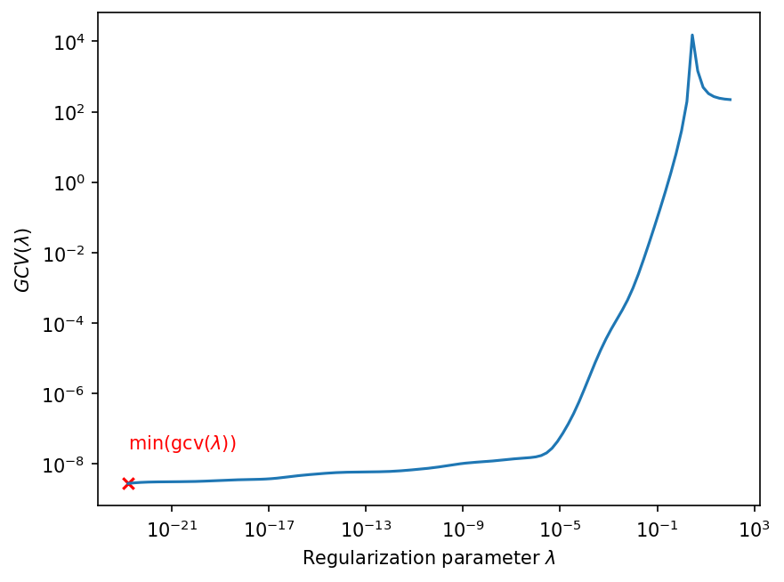
The results of the GCV optimization shows that GCV does not work for this inversion problem.

fig, ax = gcv.plot_gcv()

gcvs = [gcv.gcv(beta) for beta in gcv.lambdas]

# anotate minimum GCV value point
ax.text(gcv.lambdas[0], gcv.gcv(gcv.lambdas[0]) * 10, "min(gcv($\\lambda$))", color="r");