Note

This page was generated from docs/notebooks/inversion/tomography_synthetic.ipynb.

Tomographic Reconstruction (synthetic data)

Here, we calculate reconstructed images from a ray-traced image (synthetic data) with the L-curve criterion, and evaluate the tomography result with true solution (phantom).

from pathlib import Path

import numpy as np
from matplotlib import pyplot as plt
from mpl_toolkits.axes_grid1 import ImageGrid
from numpy.lib.format import open_memmap
from numpy.typing import NDArray
from raysect.optical import Point3D, Spectrum, Vector3D, World

from cherab.phix.inversion import Lcurve
from cherab.phix.plasma import import_plasma
from cherab.phix.tools import profile_1D_to_2D, profile_2D_to_1D
from cherab.phix.tools.raytransfer import import_phix_rtc
from cherab.phix.tools.visualize import show_phix_profiles

plt.rcParams["figure.dpi"] = 150

# Path diffinition
POWER_DATA = Path().cwd().parent / "data" / "synthetic_data" / "2020_07_25_01_51_55" / "Power.npy"
SVD_DIR = (
    Path().cwd().parent.parent.parent / "output" / "RTM" / "2022_12_13_00_49_29" / "w_laplacian"
)

# Create scene objects
world = World()
plasma, eq = import_plasma(world)
rtc = import_phix_rtc(world, equilibrium=eq)

loading plasma (data from: phix10)...

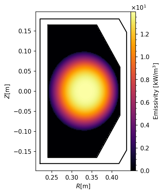
Construct the \(\text{H}_\alpha\) emissivity 2D profile

To compare the reconstructed emissivity to true one, we calculate true emissivity from PHiX plasma object.

models = [i for i in plasma.models]
print(models)

[<PlasmaModel - Bremsstrahlung>,
 <ExcitationLine: element=hydrogen, charge=0, transition=(3, 2)>,
 <ExcitationLine: element=hydrogen, charge=0, transition=(4, 2)>,
 <ExcitationLine: element=hydrogen, charge=0, transition=(5, 2)>,
 <ExcitationLine: element=hydrogen, charge=0, transition=(6, 2)>,
 <RecombinationLine: element=hydrogen, charge=0, transition=(3, 2)>,
 <RecombinationLine: element=hydrogen, charge=0, transition=(4, 2)>,
 <RecombinationLine: element=hydrogen, charge=0, transition=(5, 2)>,
 <RecombinationLine: element=hydrogen, charge=0, transition=(6, 2)>]

# set constants
nr = rtc.material.grid_shape[0]
nz = rtc.material.grid_shape[2]
rmin = rtc.material.rmin
zmin = rtc.transform[2, 3]
rmax = rmin + rtc.material.dr * nr
zmax = zmin + rtc.material.dz * nz

xrange = np.linspace(rmin, rmax, nr)
yrange = np.linspace(zmin, zmax, nz)

Halpha = (655.6, 656.8)
Halpha_model = [models[1], models[5]]
emissivity = np.zeros((nr, nz))
spectrum_bins = 50

# sample emissivity
for i, x in enumerate(xrange):
    for j, y in enumerate(yrange):
        for model in Halpha_model:
            emissivity[i, j] += (
                model.emission(
                    Point3D(x, 0.0, y),
                    Vector3D(0, 1, 0),
                    Spectrum(Halpha[0], Halpha[1], spectrum_bins),
                ).total()
                * 4.0
                * np.pi
            )  # [W/m^3/str] -> [W/m^3]

Show the \(\text{H}_\alpha\) emissivity profile

fig, ax = show_phix_profiles(emissivity * 1e-3, rtc=rtc, clabel="Emissivity [kW/m$^3$]")

Convert 2D array to 1D array corresponding to the ray-transfer object size.

emissivity_1d = profile_2D_to_1D(emissivity, rtc=rtc)

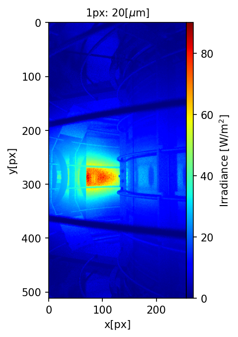
Load synthetic power data

Load the ray-traced camera image to use it as tomography data

# load image
data = np.load(POWER_DATA)

# show
fig = plt.figure()
grids = ImageGrid(fig, 111, nrows_ncols=(1, 1), cbar_mode="single", cbar_pad=0.0)
mappable = grids[0].imshow(data.T / (20e-6) ** 2, cmap="jet")
cbar = plt.colorbar(mappable, cax=grids.cbar_axes[0])
cbar.set_label("Irradiance [W/m$^2$]")
grids[0].set_xlabel("x[px]")
grids[0].set_ylabel("y[px]")
grids[0].set_title("1px: 20[$\\mu$m]", size=10);

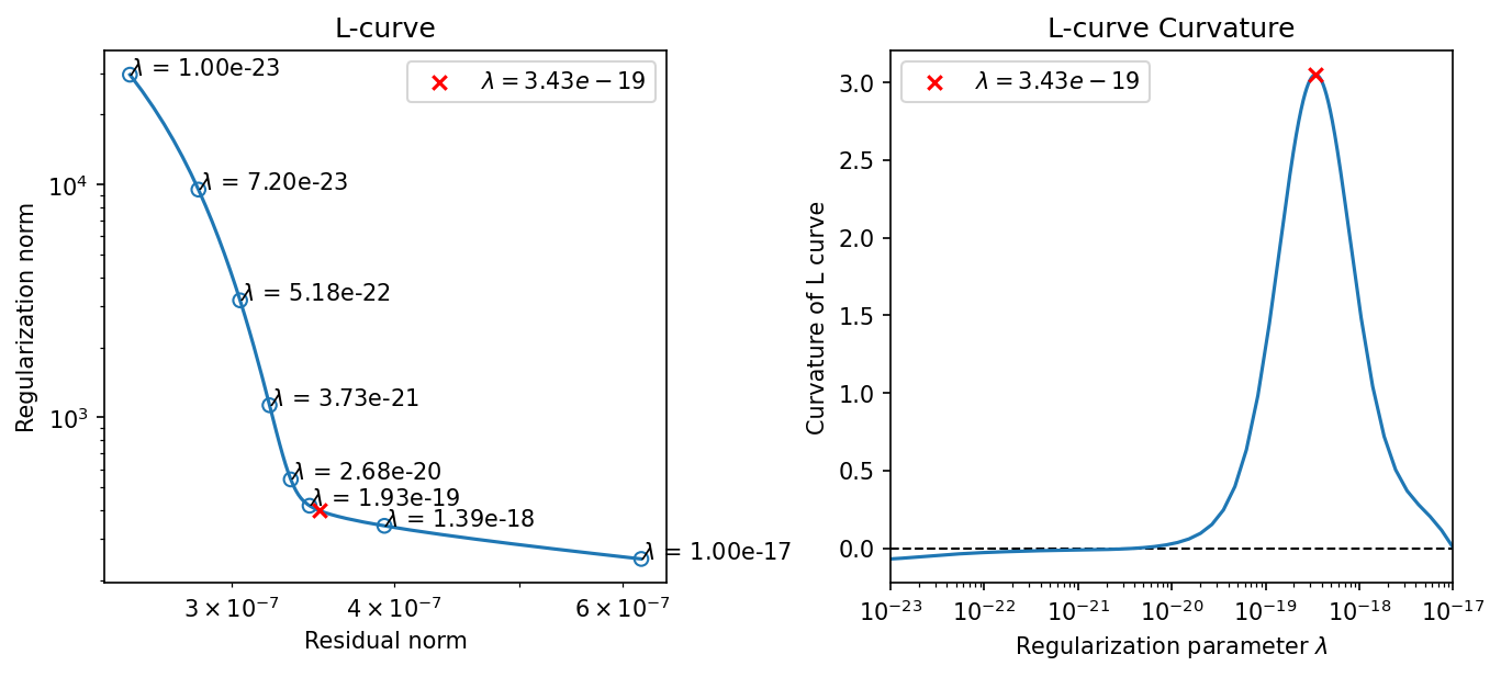
Tomographic Reconstruction with L-curve criterion

Load SVD components using numpy.memmap array.

s = open_memmap(SVD_DIR / "s.npy")
u = open_memmap(SVD_DIR / "u.npy")
vh = open_memmap(SVD_DIR / "vh.npy")
inversion_base_vectors = open_memmap(SVD_DIR / "L_inv_V.npy")

Instantiate Lcurve class

lcurve = Lcurve(s, u, vh, data, inversion_base_vectors=inversion_base_vectors)
lcurve.lambdas = 10 ** np.linspace(-23, -17)

Execute L-curve optimization

lcurve.optimize(itemax=5)

completed the optimization (iteration times : 5)

Plot L-curve and its curvature. The red cross point corresponds to the optimal regularization parameter.

fig, axes = plt.subplots(1, 2, constrained_layout=True, figsize=(9, 4))

# L-curve plot
lcurve.plot_L_curve(fig=fig, axes=axes[0], scatter_plot=8)
axes[0].set_title("L-curve")
axes[0].legend()

# curvature plot
lcurve.plot_curvature(fig=fig, axes=axes[1])
axes[1].set_title("L-curve Curvature")
axes[1].legend();

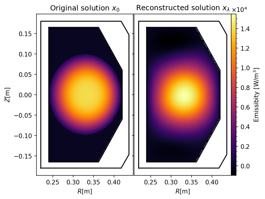
Compare the reconstructed emissivity and true (original) one.

fig, axes = show_phix_profiles(
    [emissivity, profile_1D_to_2D(lcurve.optimized_solution() * 4.0 * np.pi, rtc=rtc)],
    clabel="Emissibity [W/m$^3$]",
)
axes[0].set_title("Original solution $x_0$")
axes[1].set_title("Reconstructed solution $x_\\lambda$");

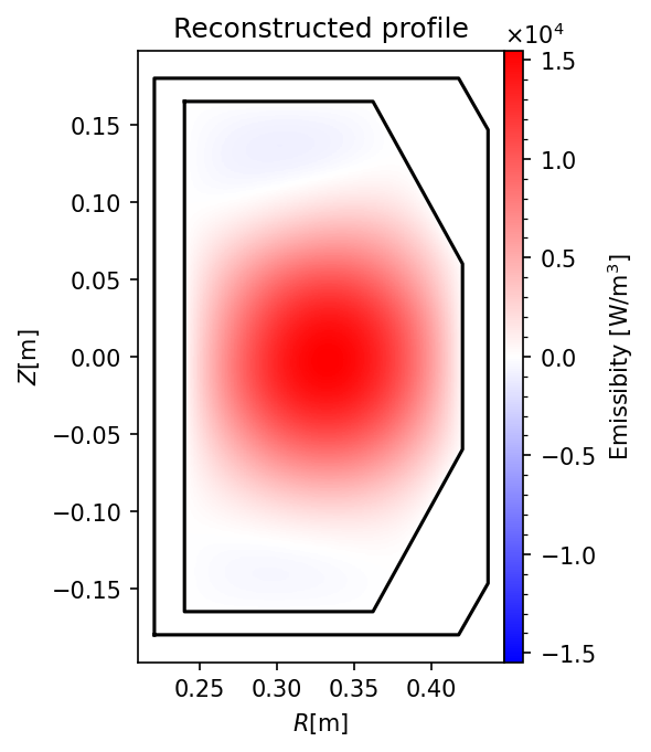
Show only the reconstructed image with negative values at the optimal regularization parameter.

fig, axes = show_phix_profiles(
    [profile_1D_to_2D(lcurve.inverted_solution(lcurve.lambda_opt) * 4.0 * np.pi, rtc=rtc)],
    clabel="Emissibity [W/m$^3$]",
    cmap="bwr",
    plot_mode="centered",
)
axes[0].set_title("Reconstructed profile");

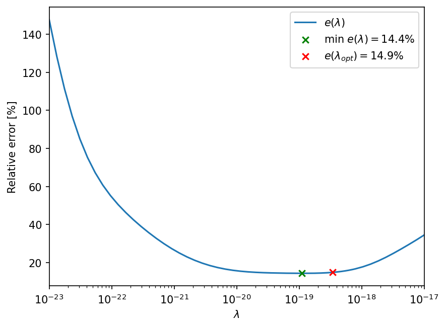
Deffinition of the relative error function

To evaluate the optimal inversion solution, let us define the following error function:

\[e(\lambda) \equiv \frac{||x_0 - x_\lambda||}{||x_0||} \times 100 \ [\%].\]

def error(x_0: NDArray, lcurve: Lcurve, beta: float) -> np.floating:
    """Compute Relative error value

    Parameters
    ----------
    x_0 : NDArray 1D
        True solution vector [W/m^3]
    lcurve : Lcurve
        Lcurve class instance
    beta : float
        regularization parameter

    Return
    ------
    float
        relative error percentage
    """
    return (
        100.0
        * np.linalg.norm(x_0 - lcurve.inverted_solution(beta) * 4.0 * np.pi)
        / np.linalg.norm(x_0)
    )

lambdas = lcurve.lambdas
residuals = [error(emissivity_1d, lcurve, beta) for beta in lambdas]
min_index = np.argmin(residuals)
fig, axes = plt.subplots()
axes.semilogx(lambdas, residuals, label="$e(\\lambda)$", zorder=-1)
axes.scatter(
    lambdas[min_index],
    residuals[min_index],
    marker="x",
    color="g",
    label=f"min $e(\\lambda) = ${residuals[min_index]:.1f}%",
)
axes.scatter(
    lcurve.lambda_opt,
    error(emissivity_1d, lcurve, lcurve.lambda_opt),
    marker="x",
    color="r",
    label=f"$e(\\lambda_{{opt}})= ${error(emissivity_1d, lcurve, lcurve.lambda_opt):.1f}%",
)
axes.legend()
axes.set_xlabel("$\\lambda$")
axes.set_ylabel("Relative error [%]")
axes.set_xlim(lambdas.min(), lambdas.max());

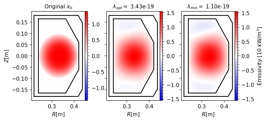
Compare inverted solution with original and minimam error solutions. To evaluate positive and negative anomalies around a center 0, we take the centered colormap to show the profiles.

fig, grids = show_phix_profiles(
    [
        emissivity * 1e-4,
        profile_1D_to_2D(lcurve.optimized_solution() * 4.0 * np.pi, rtc=rtc) * 1e-4,
        profile_1D_to_2D(lcurve.inverted_solution(lambdas[min_index]) * 4.0 * np.pi, rtc) * 1e-4,
    ],
    axes_pad=0.5,
    cbar_mode="each",
    cmap="bwr",
    plot_mode="centered",
)

grids.cbar_axes[2].set_ylabel("Emissivity [10 kW/m$^3$]")

grids[0].set_title("Original $x_0$", size=10)
grids[1].set_title(f"$\\lambda_{{opt}} =$ {lcurve.lambda_opt:.2e}", size=10)
grids[2].set_title(f"$\\lambda_{{min}} =$ {lambdas[min_index]:.2e}", size=10)
fig.set_size_inches(7, 7)

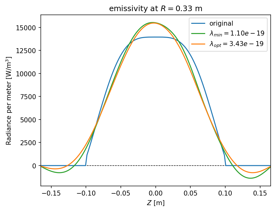
Vertical cross-section of solutions

z = (
    np.linspace(
        -165 + rtc.material.dz * 0.5, 165 - rtc.material.dz * 0.5, rtc.material.grid_shape[2]
    )
    * 1e-3
)
r = np.linspace(
    rtc.material.rmin + rtc.material.dr * 0.5,
    rtc.material.rmin + rtc.material.dr * rtc.material.grid_shape[0] - rtc.material.dr * 0.5,
    rtc.material.grid_shape[0],
)
minimum_solution = profile_1D_to_2D(lcurve.inverted_solution(lambdas[min_index]), rtc) * 4.0 * np.pi
optimized_solution = profile_1D_to_2D(lcurve.optimized_solution(), rtc) * 4.0 * np.pi
plt.plot(z, emissivity[45, :], c="C0", label="original")
plt.plot(z, minimum_solution[45, :], c="C2", label=f"$\\lambda_{{min}} = {lambdas[min_index]:.2e}$")
plt.plot(
    z, optimized_solution[45, :], c="C1", label=f"$\\lambda_{{opt}} = {lcurve.lambda_opt:.2e}$"
)
plt.plot([z.min(), z.max()], [0, 0], "--", color="k", zorder=-1, linewidth=0.75)
plt.legend()
plt.xlim(z.min(), z.max())
plt.title(f"emissivity at $R = {r[45]:.2f}$ m")
plt.xlabel("$Z$ [m]")
plt.ylabel("Radiance per meter [W/m$^3$]");