Note

This page was generated from docs/notebooks/observer/rgb_convert.ipynb.

Convert RGB to incident power

Diffinition

As usual, a fast visible camera generates R, G, B values at each pixel which has a specific sensitivity to the wavelength. So, To evaluate the tomographic emission profile with the physical energy unit, we need to estimate the incident power into each pixel from the RGB value.

Each pixel data captured by the fast camera installed at PHiX, Phantom LAB 110, follows the simplified formula below:

\[\begin{align} \text{DN} = \frac{t}{6.15\times 10^{-9} A}\int_{\mathbb{R}} \mathrm{d}\lambda\; S(\lambda)P(\lambda), \end{align}\]

where,

• DN: sensor response (in digital number, 12bits, from 0-4095),

• \(t\): exposure time set in camera (in second).

• \(A\): the area of laser beam throwing on the sensor array ( in \(\mathrm{m}^2\)),

• \(\lambda\): wavelength (in nm),

• \(S(\lambda)\): spectral response at a specific wavelength (in A/W),

• \(P(\lambda)\): the incident spectral power (in watt per nm).

Considering only \(\text{H}_\alpha\), \(\text{H}_\beta\) and \(\text{H}_\gamma\) spectral incident power \(P(\lambda)\) because they dominates the PHiX experiments, we can calculate R value as follows:

\[\begin{split}\begin{align} R & = \frac{t \times 10^9}{6.15 A}\sum_{x=\alpha, \beta, \gamma} \int_{\varDelta\lambda_x} \mathrm{d}\lambda S_R(\lambda)P(\lambda)\\ &\approx \frac{t \times 10^9}{6.15 A}\sum_{x=\alpha, \beta, \gamma}S_R(\lambda_x) P_x, \left( \text{where }P_x \equiv \int_{\varDelta \lambda_x}\mathrm{d}\lambda P(\lambda) \right) \end{align}\end{split}\]

where, \(S_R\) is the spectral response of R filter and \(\varDelta\lambda_x\) is a wavelength range near the corresponding emission line. The last line assumes that \(S_R\) is constant with \(S_R(\lambda_x)\) around the corresponding line emission.

Applying the above expression to the other color value (G, B), the following linear equation is derived:

\[\begin{split}\begin{pmatrix} R\\ G\\ B\\ \end{pmatrix} =\frac{t \times 10^9}{6.15 A} \begin{pmatrix} S_R(\lambda_\alpha) & S_R(\lambda_\beta) & S_R(\lambda_\gamma)\\ S_G(\lambda_\alpha) & S_G(\lambda_\beta) & S_G(\lambda_\gamma)\\ S_B(\lambda_\alpha) & S_B(\lambda_\beta) & S_B(\lambda_\gamma)\\ \end{pmatrix} \begin{pmatrix} P_\alpha\\ P_\beta\\ P_\gamma\\ \end{pmatrix}.\end{split}\]

Therefore, solving the above linear equation allows us to calculate each incident power.

from pathlib import Path

import numpy as np
from matplotlib import pyplot as plt
from mpl_toolkits.axes_grid1 import ImageGrid

from cherab.phix.observer.fast_camera.colour import filter_b, filter_g, filter_r, plot_RGB_filter

RGB_DATA = Path().cwd().parent / "data" / "experiment" / "shot_17393_raw.npy"

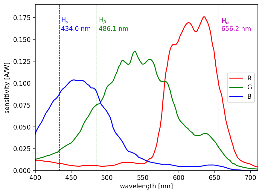
Plot the RGB sensitivity with \(\text{H}_\alpha\), \(\text{H}_\beta\), \(\text{H}_\gamma\) lines

Let us plot RGB sensitivity data which is given by the company.

# wavelength corresponding to each hydrogen balmer line
H_ALPHA = (655.6 + 656.8) * 0.5
H_BETA = (485.6 + 486.5) * 0.5
H_GAMMA = (433.6 + 434.4) * 0.5

fig, ax = plt.subplots(dpi=150)
wavelengths = np.linspace(400, 710, 500)

# plot sensitivity
fig, ax = plot_RGB_filter(wavelengths, fig=fig, ax=ax)
ax.legend(loc="center right")

# plot hydrogen balmers
for wavelength, color, symbol in zip(
    [H_ALPHA, H_BETA, H_GAMMA], ["m", "g", "b"], ["\\alpha", "\\beta", "\\gamma"]
):
    ax.plot([wavelength, wavelength], [0, 0.2], color=color, linestyle="dashed", linewidth=0.75)
    ax.text(wavelength * 1.005, 0.16, f"$\\mathrm{{H}}_{symbol}$\n{wavelength:.1f} nm", color=color)

ax.set_ylim(0, 0.19)
ax.set_xlim(wavelengths[0], wavelengths[-1]);

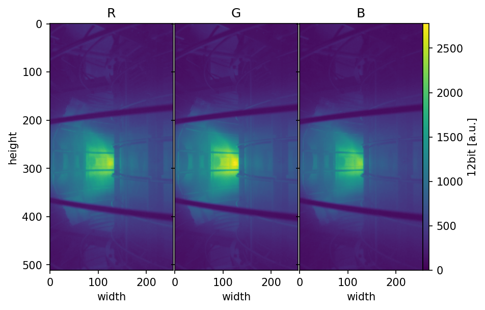
Convert 12bit RGB data

Let us convert RGB experimental image.

Firstly let’s show the original image data.

# Load data
rgb_image = np.load(RGB_DATA)

# show image
fig = plt.figure(dpi=150)
grids = ImageGrid(fig, 111, (1, 3), cbar_mode="single", cbar_pad=0.0, axes_pad=0.02)
for i, label in enumerate(["R", "G", "B"]):
    grids[i].imshow(rgb_image[:, :, i], cmap="viridis", vmax=np.amax(rgb_image), vmin=0)
    grids[i].set_title(label)
    grids[i].set_xlabel("width")
grids[0].set_ylabel("height")
cbar = plt.colorbar(grids[0].images[-1], cax=grids.cbar_axes[0])
cbar.set_label("12bit [a.u.]")

Then, construct a spectrum \(\rightarrow\) RGB values matrix.

# Spectrum -> RGB matrix [A]
spectrum_to_rgb = np.array(
    [
        [filter_r(H_ALPHA), filter_r(H_BETA), filter_r(H_GAMMA)],
        [filter_g(H_ALPHA), filter_g(H_BETA), filter_g(H_GAMMA)],
        [filter_b(H_ALPHA), filter_b(H_BETA), filter_b(H_GAMMA)],
    ],
    dtype=np.float64,
)

Solve the linear equation at each pixel.

dt = 99e-6  # [sec]
A_1px = 20e-6 * 20e-6  # [m^2]

spectrum_image = np.zeros_like(rgb_image, dtype=np.float64)

for x in range(rgb_image.shape[0]):
    for y in range(rgb_image.shape[1]):
        spectrum_image[x, y, :] = np.linalg.solve(
            spectrum_to_rgb, rgb_image[x, y, :] * 6.15e-9 * A_1px / dt
        )

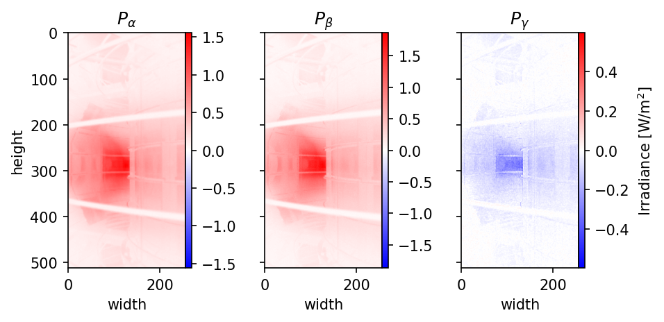
Show the solution

from matplotlib.colors import CenteredNorm

fig = plt.figure(dpi=150)
grids = ImageGrid(fig, 111, (1, 3), cbar_mode="each", cbar_pad=0.0, axes_pad=0.7)
for i, symbol in enumerate(["\\alpha", "\\beta", "\\gamma"]):
    grids[i].imshow(spectrum_image[:, :, i] / A_1px, cmap="bwr", norm=CenteredNorm())
    grids[i].set_title(f"$P_{symbol}$")
    grids[i].set_xlabel("width")
    cbar = plt.colorbar(grids[i].images[0], cax=grids.cbar_axes[i])
grids[0].set_ylabel("height")
cbar.set_label("Irradiance [W/m$^2$]")

Plot each irradiance values at width 128 px.

for i, color, symbol in zip(range(3), ["m", "g", "b"], ["\\alpha", "\\beta", "\\gamma"]):
    plt.plot(spectrum_image[:, 128, i] / A_1px, color=color, label=f"$P_{symbol}$", zorder=1)
plt.plot([0, 512], [0, 0], "--k", linewidth=0.7, zorder=0)
plt.xlim(0, 512)
plt.legend()
plt.xlabel("height [px]")
plt.ylabel("Irradiance [W/m$^2$]")
plt.title("at width: 128[px]");

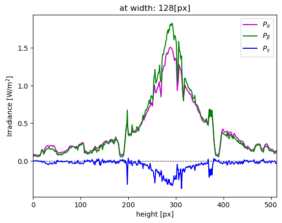
The results show that \(P_\gamma\) reconstruction did not work well because the negative values dominates. However, the rest of the solutions are relatively reconstructed well.